3 Projects Well Suited For

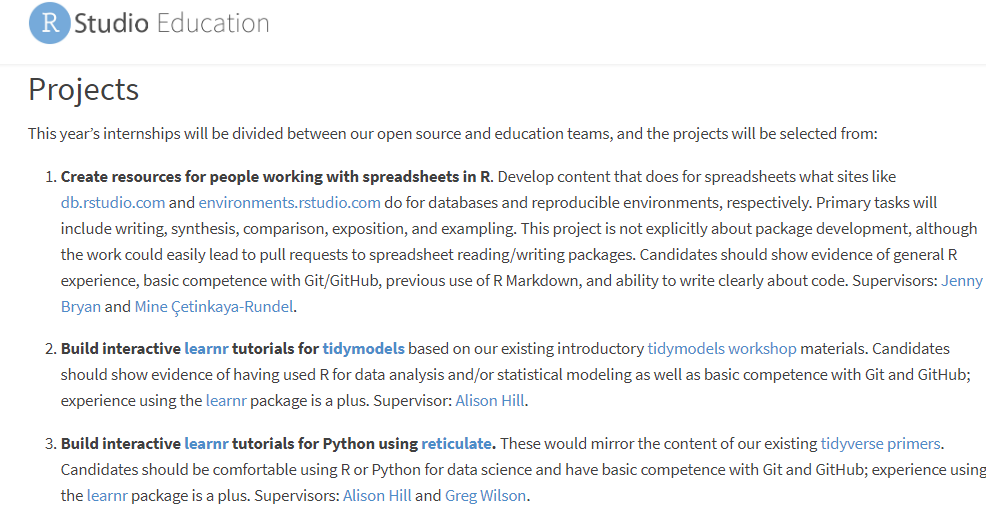
3.1 Create resources for people working with spreadsheets in R

What better way to show I am suited for a project than to give a hands-on example? See the code below for a use-case using googlesheets4(Bryan 2020).

First I will go ahead and import every package in the tidyverse(Wickham 2019):

library(tidyverse)

We will be importing the following spreadsheet:

spreadsheet_url <- "https://docs.google.com/spreadsheets/d/1_zRBFrB1au7qhxuDDfDuh_bPLGd6RLrwOL5oQ3sBBX4/edit?usp=sharing"

Before importing the data, let’s use tictoc (Izrailev 2014) to measure how long each step takes. I am using tic() to start the time for both the total execution time and for the step reading the data in. After importing the data we will run toc() to get the execution time for that step.

library(tictoc)
tic('Total section 3 runtime')
tic('Read googlesheets data')

Now let’s import the googlesheets4 and read a spreadsheet I made for this internship application, specifying the sheet called coinmetrics_preview inside the function read_sheet():

library(googlesheets4)
googlesheets_data <- read_sheet(spreadsheet_url, sheet = 'coinmetrics_preview') %>% as.data.frame() # won't work with Github Actions

toc()

## Read googlesheets data: 48.4 sec elapsed

Let’s take a peek at the first 1,000 rows using DT::datatable() (Xie, Cheng, and Tan 2019)

library(DT)
datatable(head(googlesheets_data,1000),  style = "default", 
          options = list(scrollX = TRUE, pageLength=5,dom='t'), rownames = F)

This data is sourced from the website coinmetrics.io

How many rows in the dataset?

nrow(googlesheets_data)

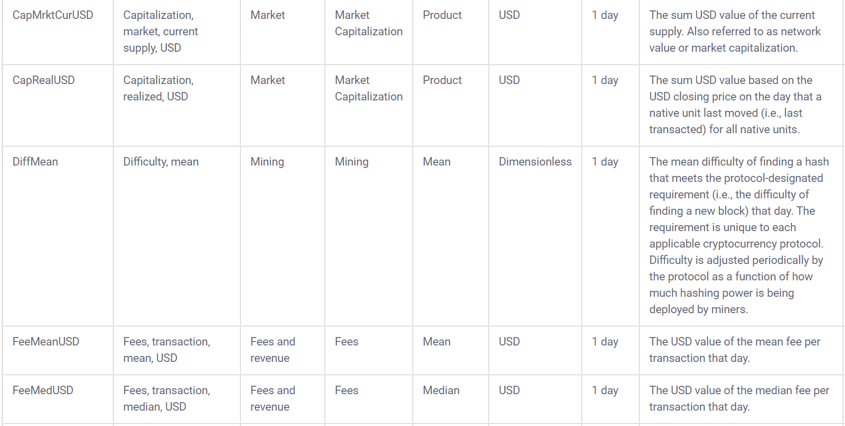
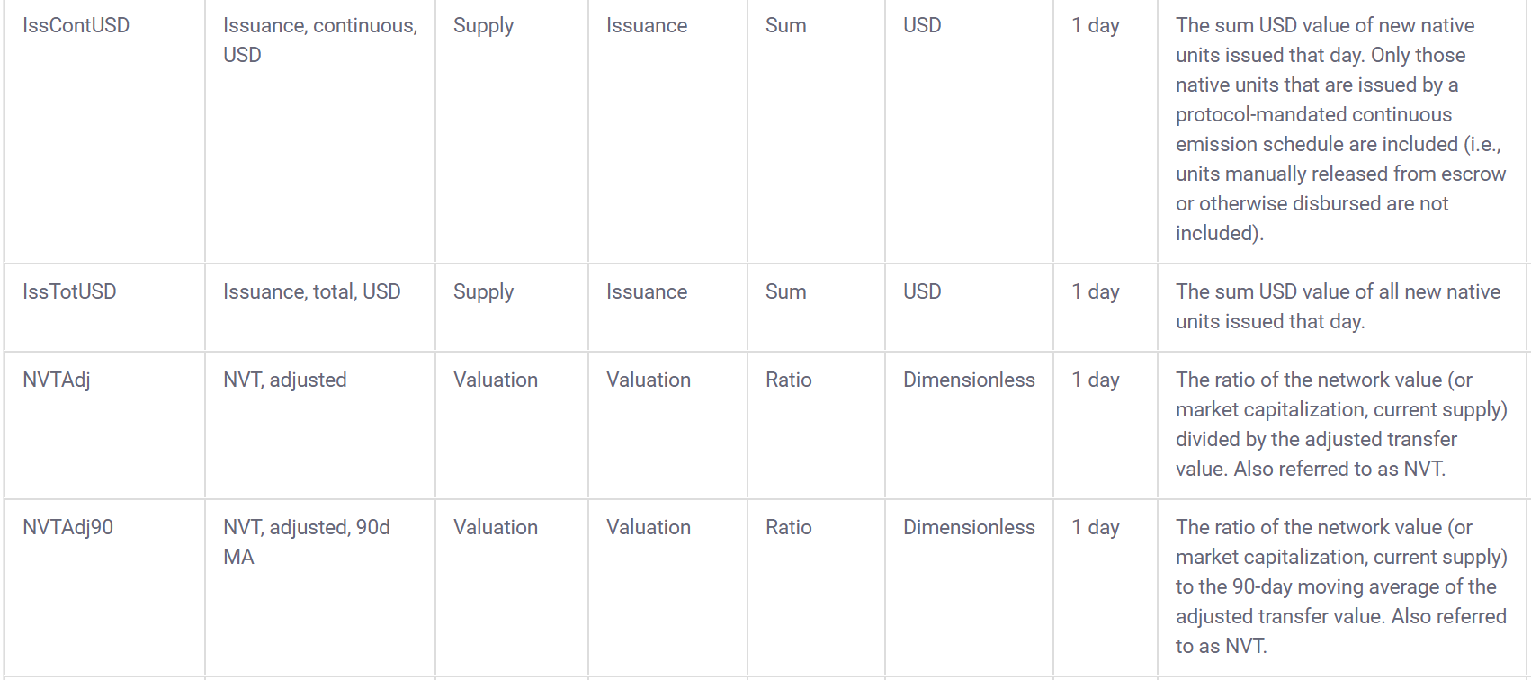
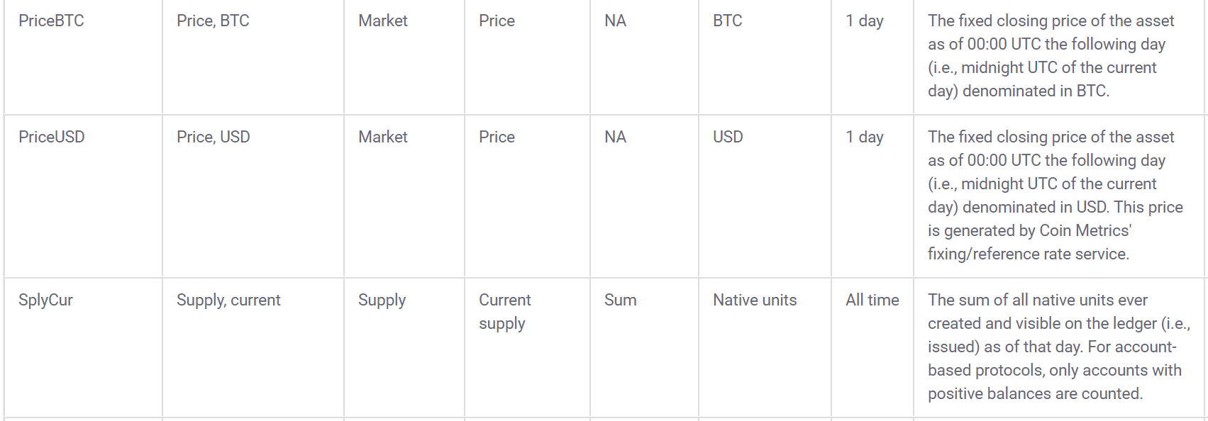
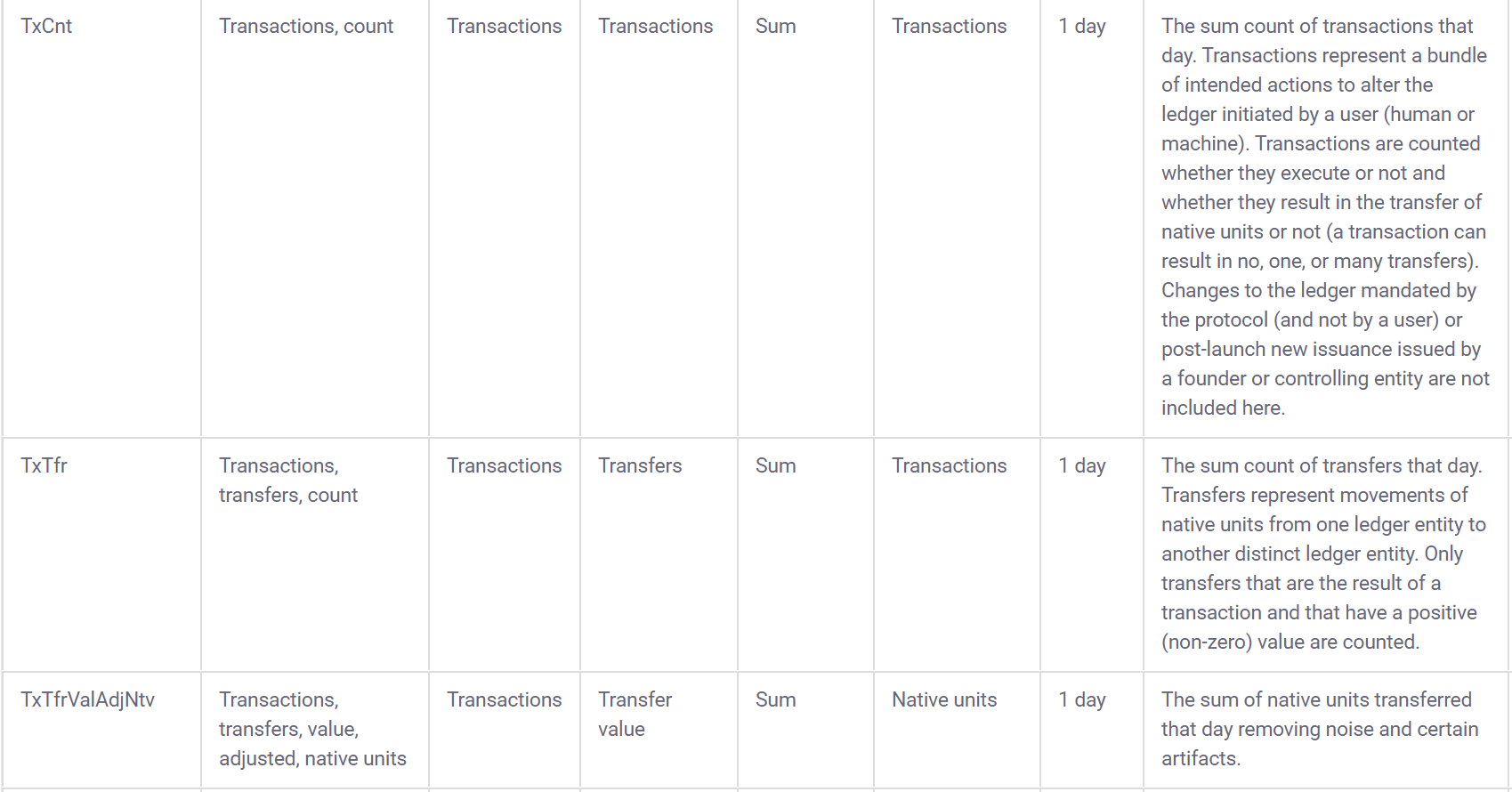
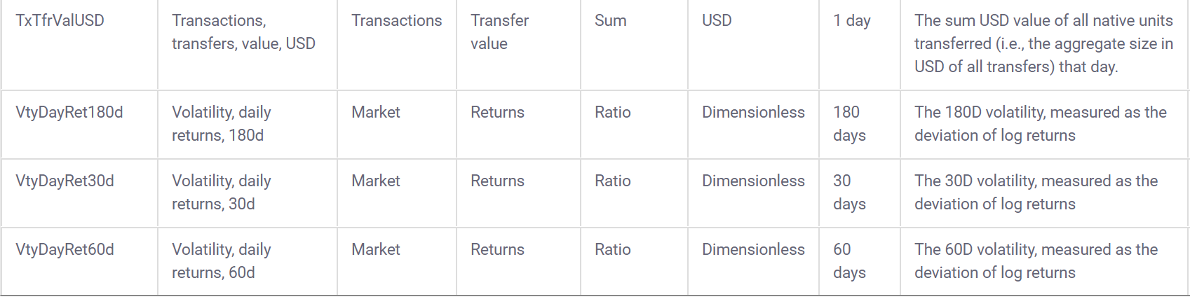
## [1] 11995

Coinmetrics also provides a data dictionary to go along with the data:

3.2 Build interactive learnr tutorials for tidymodels

3.2.1 Data Prep

Using the data from coinmetrics, I will create a predictive model to forecast the percentage change in price over time.

First, I will import a package that I am making that is still in development PredictCrypto:

library(PredictCrypto)

(this is an in-development tool that I will use for a research paper I am working on)

I attended the two day building tidy tools workshop working with Charlotte and Hadley at RStudio::conf 2020 and I am comfortable writing packages in R as well as using testthat and showing code coverage for a repository.

Here is the GitHub Pages environment associated with the repository:

I am going to convert the column names from CamelCase to snake_case using the janitor(Firke 2020) package because the functions in my package use snake_case and I want to avoid mixing the two:

Before:

##  [1] "Date"            "Symbol"          "AdrActCnt"       "BlkCnt"          "BlkSizeByte"     "BlkSizeMeanByte" "CapMVRVCur"     
##  [8] "CapMrktCurUSD"   "CapRealUSD"      "DiffMean"        "FeeMeanNtv"      "FeeMeanUSD"      "FeeMedNtv"       "FeeMedUSD"      
## [15] "FeeTotNtv"       "FeeTotUSD"       "HashRate"        "IssContNtv"      "IssContPctAnn"   "IssContUSD"      "IssTotNtv"      
## [22] "IssTotUSD"       "NVTAdj"          "NVTAdj90"        "PriceBTC"        "PriceUSD"        "ROI1yr"          "ROI30d"         
## [29] "SplyCur"         "TxCnt"           "TxTfrCnt"        "TxTfrValAdjNtv"  "TxTfrValAdjUSD"  "TxTfrValMeanNtv" "TxTfrValMeanUSD"
## [36] "TxTfrValMedNtv"  "TxTfrValMedUSD"  "TxTfrValNtv"     "TxTfrValUSD"     "VtyDayRet180d"   "VtyDayRet30d"    "VtyDayRet60d"   
## [43] "DateTimeUTC"

library(janitor)
googlesheets_data <- clean_names(googlesheets_data)

After:

##  [1] "date"                "symbol"              "adr_act_cnt"         "blk_cnt"             "blk_size_byte"       "blk_size_mean_byte" 
##  [7] "cap_mvrv_cur"        "cap_mrkt_cur_usd"    "cap_real_usd"        "diff_mean"           "fee_mean_ntv"        "fee_mean_usd"       
## [13] "fee_med_ntv"         "fee_med_usd"         "fee_tot_ntv"         "fee_tot_usd"         "hash_rate"           "iss_cont_ntv"       
## [19] "iss_cont_pct_ann"    "iss_cont_usd"        "iss_tot_ntv"         "iss_tot_usd"         "nvt_adj"             "nvt_adj90"          
## [25] "price_btc"           "price_usd"           "roi1yr"              "roi30d"              "sply_cur"            "tx_cnt"             
## [31] "tx_tfr_cnt"          "tx_tfr_val_adj_ntv"  "tx_tfr_val_adj_usd"  "tx_tfr_val_mean_ntv" "tx_tfr_val_mean_usd" "tx_tfr_val_med_ntv" 
## [37] "tx_tfr_val_med_usd"  "tx_tfr_val_ntv"      "tx_tfr_val_usd"      "vty_day_ret180d"     "vty_day_ret30d"      "vty_day_ret60d"     
## [43] "date_time_utc"

Now that I imported the PredictCrypto package and the data is in snake_case, I can use the function calculate_percent_change() to create the target variable to predict. Before I can do that however, I need one more adjustment to the date/time fields, so let’s do that using the anytime(Eddelbuettel 2020) package:

library(anytime)
googlesheets_data$date <- anytime(googlesheets_data$date)
googlesheets_data$date_time_utc <- anytime(googlesheets_data$date_time_utc)

Now I can use the function calculate_percent_change() to calculate the % change of the price of each cryptocurrency and add a new column target_percent_change to each row, which will represent the percentage change in price for the 7 day period that came after that data point was collected:

exercise_data <- PredictCrypto::calculate_percent_change(googlesheets_data, 7, 'days')

Let’s take a peek at the new field:

tail(exercise_data$target_percent_change, 10)

##  [1] -21.577214 -22.986805 -14.995782  -3.220387  -8.205419 -16.015721 -16.911053 -12.801616 -16.444769 -17.383620

I could easily change this to a 14 day period:

calculate_percent_change(googlesheets_data, 14, 'days') %>% tail(10) %>% select(target_percent_change)

##       target_percent_change
## 10784             -16.13764
## 10785             -13.74175
## 10786             -16.13759
## 10787             -10.74085
## 10788             -17.04613
## 10789             -23.68376
## 10790             -33.13588
## 10791             -31.61660
## 10792             -35.65145
## 10793             -29.77259

Or a 24 hour period:

calculate_percent_change(googlesheets_data, 24, 'hours') %>% tail(10) %>% select(target_percent_change)

##       target_percent_change
## 10849             -3.215170
## 10850              2.203778
## 10851             -1.520398
## 10852              7.513390
## 10853             -6.282062
## 10854             -5.897307
## 10855            -10.042910
## 10856              1.571641
## 10857             -2.066301
## 10858             -2.626944

Disclaimer: Most of the code to follow was built using the content made available by Allison Hill from the RStudio::conf2020 intro to machine learning workshop and was not code I was familiar with before writing it for this internship application:

https://education.rstudio.com/blog/2020/02/conf20-intro-ml/

https://conf20-intro-ml.netlify.com/materials/01-predicting/

3.2.2 Feature scaling

tic('Feature scaling')

Before getting started on the predictive modeling section, it’s a good idea for us to scale the numeric data in our dataset. Some of the fields in the dataset are bound to have dramatically different ranges in their values:

mean(exercise_data$roi30d, na.rm=T)

## [1] 20.22271

mean(exercise_data$cap_mrkt_cur_usd)

## [1] 17191065374

This can be problematic for some models (not every model has this issue), and the difference in the magnitude of the numbers could unfairly influence the model to think that the variable with the larger numbers is more statistically important than the one with the lesser values when that might not actually be true.

For feature scaling, we need to do two things:

1. Center the data in every column to have a mean of zero

2. Scale the data in every column to have a standard deviation of one

The recipes (Kuhn and Wickham 2020) package is a very useful package for pre-processing data before doing predictive modeling, and it allows us to center the way we do our data engineering around the independent variable we are looking to predict, which in our case is the target_percent_change. We can make a recipe which centers all numeric fields in the data using step_center() and then scale them using step_scale(). We will also remove the symbol column from the recipe using step_rm() because we don’t want to use it for the predictions but we don’t want to remove it from the dataset either:

library(recipes)
scaling_recipe <- recipe(target_percent_change ~ ., data = exercise_data) %>%
  step_center(all_numeric()) %>% 
  step_scale(all_numeric())

Commented out step_novel(all_nominal()), step_dummy(all_nominal()), step_nz(all_predictors()) because size too large and won’t run on PC or GitHub Actions.

Now that we have made a data pre-processing recipe, let’s map it to the exercise_data dataset:

crypto_data_scaled <- scaling_recipe %>% prep(exercise_data) 
crypto_data_scaled

## Data Recipe
## 
## Inputs:
## 
##       role #variables
##    outcome          1
##  predictor         46
## 
## Training data contained 10828 data points and 3120 incomplete rows. 
## 
## Operations:
## 
## Centering for adr_act_cnt, blk_cnt, blk_size_byte, blk_size_mean_byte, cap_mrkt_cur_usd, diff_mean, ... [trained]
## Scaling for adr_act_cnt, blk_cnt, blk_size_byte, blk_size_mean_byte, cap_mrkt_cur_usd, diff_mean, ... [trained]

Now let’s use bake() to put the old dataset in the oven and get back the scaled data 🍰:

crypto_data_scaled <- crypto_data_scaled %>% bake(exercise_data)

Now the values are scaled:

head(crypto_data_scaled$cap_mrkt_cur_usd,5)  

## [1] -0.4306519 -0.4306511 -0.4306502 -0.4310321 -0.4304881

You can see the difference from the previous values:

head(exercise_data$cap_mrkt_cur_usd,5)

## [1] 86768713 86801326 86834707 71666978 93274716

toc()

## Feature scaling: 0.34 sec elapsed

3.2.3 Predictive Modeling

tic('Predictive Modeling')

We can create models using parsnip (Kuhn and Vaughan 2020), which is particularly nice because it gives a very standardized structure for a variety of models. Here’s the slightly over-complicated lm() linear regression model using parsnip:

library(parsnip)
lm_model <- linear_reg() %>%
  set_engine("lm") %>%
  set_mode("regression")

List of models to refer to: https://tidymodels.github.io/parsnip/articles/articles/Models.html

Random Forest:

random_forest_model <- rand_forest(trees = 1000) %>%
  set_engine("randomForest") %>%
  set_mode("regression")

XGBoost:

xgboost_model <- xgboost_parsnip <- boost_tree(trees=1000) %>%
  set_engine("xgboost") %>%
  set_mode("regression")

Remove the fields we will not be be using for the predictive modeling:

exercise_data <- exercise_data %>% select(-date_time_utc, -date_time, -pkDummy, -pkey, -cap_real_usd, -cap_mvrv_cur)

Before we can start fitting a predictive model, we need to create a train/test split, we can use rsample(Kuhn, Chow, and Wickham 2019) to put 80% of the data into crypto_train and 20% of the data in crypto_test:

library(rsample)

set.seed(250)
crypto_data <- initial_split(exercise_data, prop = 0.8)
crypto_train <- training(crypto_data)
crypto_test  <-  testing(crypto_data)

Compare the number of rows:

nrow(crypto_train) # 80% of rows

## [1] 8663

nrow(crypto_test) # 20% of rows

## [1] 2165

3.2.4 Fit the model:

Now we can go ahead and train/fit the models to the data:

library(modelr)
lm_fitted <- lm_model %>% fit(target_percent_change ~ ., data=crypto_train)

Random Forest:

tic('Random Forest')

random_forest_fitted <- random_forest_model %>%
  fit(target_percent_change ~ ., data = crypto_train)

toc()

## Random Forest: 141.81 sec elapsed

XGBoost:

tic('XGBoost')

xgboost_fitted <- xgboost_model %>% fit(price_usd ~ ., data=crypto_train)

toc()

## XGBoost: 19.2 sec elapsed

Use the trained model to make predictions on test data:

library(tidymodels)

lm_predictions <- predict(lm_fitted, crypto_test)

xgboost_predictions <- xgboost_fitted %>% predict(crypto_test)

Join the full dataset back to the predictions:

lm_predictions <- lm_predictions %>% bind_cols(crypto_test)

xgboost_predictions <- xgboost_predictions %>% bind_cols(crypto_test)

Get metrics:

lm_predictions %>%
  metrics(truth = target_percent_change, estimate = .pred)

## # A tibble: 3 x 3
##   .metric .estimator .estimate
##   <chr>   <chr>          <dbl>
## 1 rmse    standard     16.9   
## 2 rsq     standard      0.0357
## 3 mae     standard     11.0

xgboost_predictions %>%
  metrics(truth = target_percent_change, estimate = .pred)

## # A tibble: 3 x 3
##   .metric .estimator  .estimate
##   <chr>   <chr>           <dbl>
## 1 rmse    standard   2463.     
## 2 rsq     standard      0.00299
## 3 mae     standard    875.

3.2.5 Now make one model for each cryptocurrency.

Lots of code adapted from: https://r4ds.had.co.nz/many-models.html

First I group the data by the cryptocurrency symbol:

crypto_data_grouped <- exercise_data %>% group_by(symbol) %>% nest()

crypto_data_grouped

## # A tibble: 5 x 2
## # Groups:   symbol [5]
##   symbol data                 
##   <chr>  <list>               
## 1 ETH    <tibble [1,660 x 40]>
## 2 BTC    <tibble [3,507 x 40]>
## 3 LTC    <tibble [2,519 x 40]>
## 4 DASH   <tibble [2,206 x 40]>
## 5 BCH    <tibble [936 x 40]>

Make a helper function with the model so I can make the lm() model to apply to each cryptocurrency using purrr:

grouped_linear_model <- function(df) {
  lm(target_percent_change ~ ., data = df)
}

I could have made a more complex model here, but decided to keep things a bit simpler with linear regression

Now we can use purrr(Henry and Wickham 2019) to apply the model to each element of the grouped dataframe:

grouped_models <- map(crypto_data_grouped$data, grouped_linear_model)

The models can be added into the dataframe as nested lists. We can also add the corresponding residuals:

crypto_data_grouped <- crypto_data_grouped %>% 
  mutate(model=map(data,grouped_linear_model)) %>% 
  mutate(resids = map2(data, model, add_residuals))

Let’s look at the object again:

crypto_data_grouped

## # A tibble: 5 x 4
## # Groups:   symbol [5]
##   symbol data                  model  resids               
##   <chr>  <list>                <list> <list>               
## 1 ETH    <tibble [1,660 x 40]> <lm>   <tibble [1,660 x 41]>
## 2 BTC    <tibble [3,507 x 40]> <lm>   <tibble [3,507 x 41]>
## 3 LTC    <tibble [2,519 x 40]> <lm>   <tibble [2,519 x 41]>
## 4 DASH   <tibble [2,206 x 40]> <lm>   <tibble [2,206 x 41]>
## 5 BCH    <tibble [936 x 40]>   <lm>   <tibble [936 x 41]>

Let’s unnest the residuals to take a closer look:

resids <- unnest(crypto_data_grouped, resids)

resids %>% 
  ggplot(aes(date, resid)) +
    geom_line(aes(group = symbol), alpha = 1 / 3) + 
    geom_smooth(se = FALSE) +
    ylim(c(-20,20)) +
    facet_wrap(~symbol)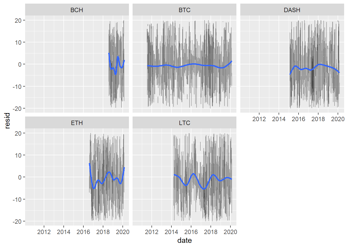

3.2.6 Add Metrics

Now we can use broom (Robinson and Hayes 2020) to get all sorts of metrics back on the models:

library(broom)
crypto_models_metrics <- crypto_data_grouped %>% mutate(metrics=map(model,broom::glance)) %>% unnest(metrics)

Sort the new tibble by the best r squared values:

crypto_models_metrics %>% arrange(-r.squared)

## # A tibble: 5 x 15
## # Groups:   symbol [5]
##   symbol data        model  resids      r.squared adj.r.squared sigma statistic  p.value    df  logLik    AIC    BIC deviance df.residual
##   <chr>  <list>      <list> <list>          <dbl>         <dbl> <dbl>     <dbl>    <dbl> <int>   <dbl>  <dbl>  <dbl>    <dbl>       <int>
## 1 BCH    <tibble [9~ <lm>   <tibble [9~     0.478         0.442  16.1      13.6 1.61e-54    37  -2378.  4833.  4998.  138706.         534
## 2 ETH    <tibble [1~ <lm>   <tibble [1~     0.300         0.279  15.1      14.5 3.62e-73    38  -5331. 10740. 10941.  285308.        1257
## 3 DASH   <tibble [2~ <lm>   <tibble [2~     0.213         0.196  15.5      12.5 1.95e-68    40  -7642. 15366. 15593.  434709.        1801
## 4 LTC    <tibble [2~ <lm>   <tibble [2~     0.193         0.179  16.8      13.7 3.99e-74    38  -9111. 18300. 18521.  595319.        2116
## 5 BTC    <tibble [3~ <lm>   <tibble [3~     0.151         0.142  12.5      15.4 1.51e-85    37 -12374. 24823. 25053.  484582.        3105

toc()

## Predictive Modeling: 163.53 sec elapsed

3.2.7 Plot Variable Importance

Now I can use the vip (Greenwell, Boehmke, and Gray 2020) package to plot the variable importance:

library(vip)

library(vip)
for (i in 1:length(crypto_models_metrics$symbol)){
  print(paste("Now showing", crypto_models_metrics$symbol[[i]], "variable importance:"))
  print(vip(crypto_models_metrics$model[[i]]))
}

## [1] "Now showing ETH variable importance:"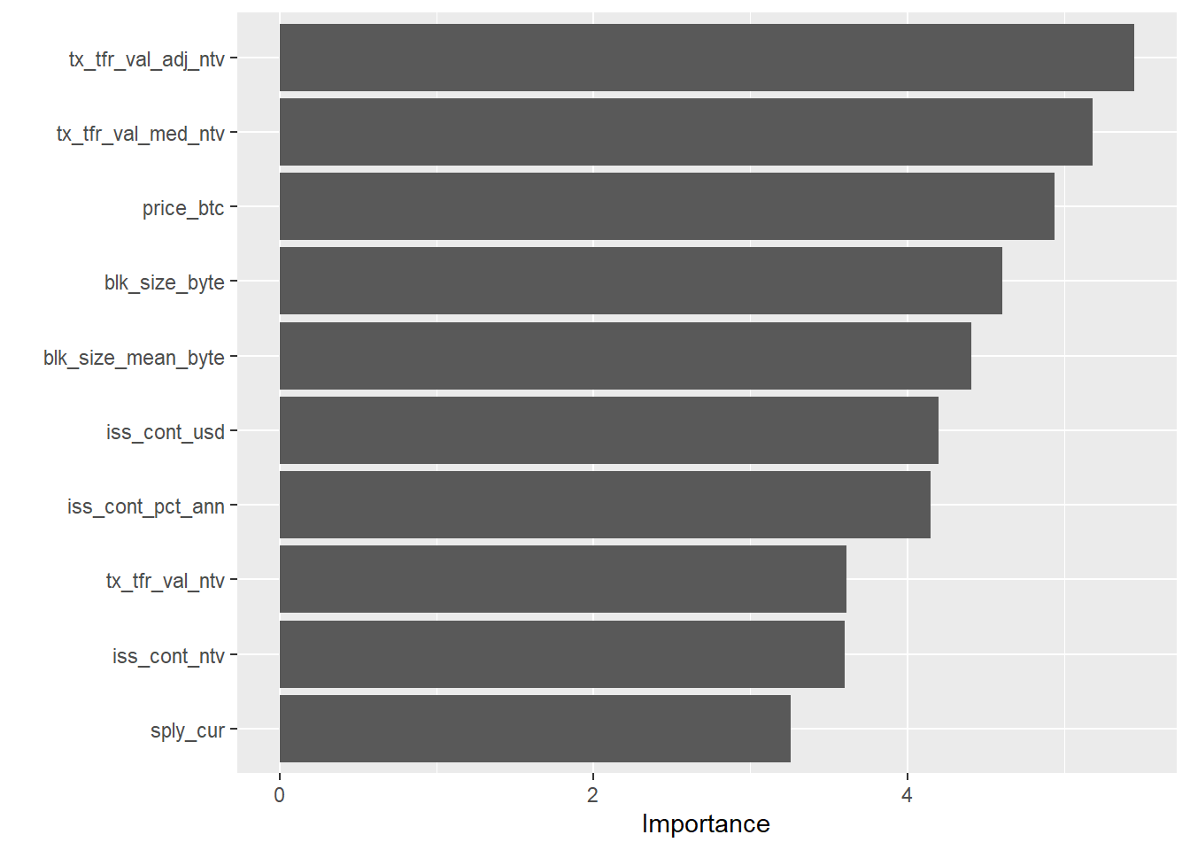

## [1] "Now showing BTC variable importance:"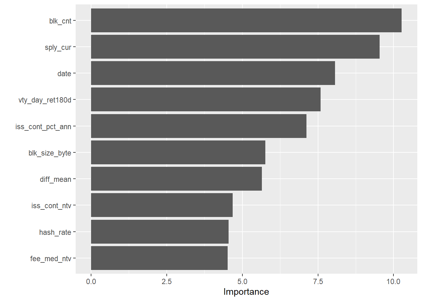

## [1] "Now showing LTC variable importance:"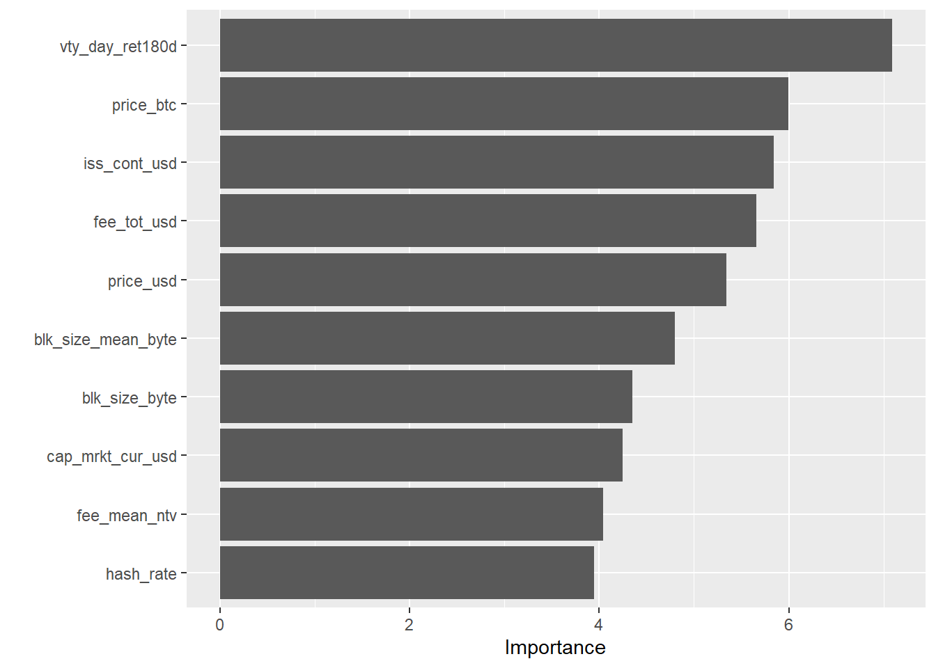

## [1] "Now showing DASH variable importance:"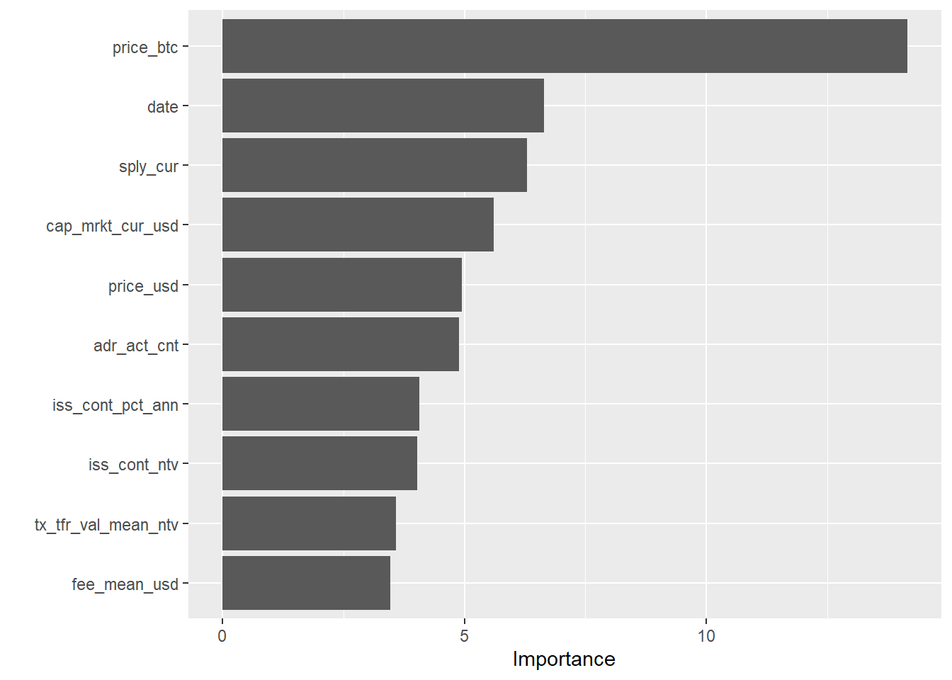

## [1] "Now showing BCH variable importance:"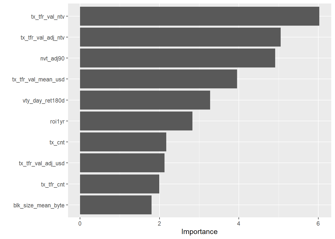

3.2.8 If I were to keep going…

Here are some of the next steps I would take if I were to keep going with this analysis:

1. How much better do the models get if we add timeseries components like Moving Averages?

2. Use parsnip + purrr to iterate through lots of predictive models rather than just applying a simple lm() model to each.

3. How much better do the models get with hyperparameter tuning? I would use dials since it’s a part of tidymodels.

4. Visualize the best model before and after parameter tuning and then do the same with the worst performing model.

5. I would also go back to the train/test split and use 10-fold cross validation instead.

3.3 Build interactive learnr tutorials for Python using reticulate

I think I could be a great fit for the third project listed related to creating learnr tutorials for Python using reticulate. I have a fair amount of experience in Python, but it’s never really clicked very much for as much as R in the past, and I am looking to step-up my Python skills. My Master’s in Data Science will work with Python a lot, and people immediately ask if I make tutorials in Python when I show them the R tutorials I have made, so this would be a great one for me to work on. I am also constantly told that Python is better than R for the incorrect reasons, and being more of an expert in Python would certainly help me debunk that myth when someone makes that argument.

I am very familiar with the reticulate package and I have used it in the past in an RMarkdown file to make automated cryptocurrency trades through a Python package shrimpy-python, which worked really well: https://github.com/shrimpy-dev/shrimpy-python

Since I have already demonstrated my familiarity with learnr tutorials in the previous section, I did not make a very extensive example here, but instead created a learnr tutorial with a Python code chunk instead:

Return the total runtime of all of the examples above:

toc()

## Total section 3 runtime: 215.46 sec elapsed

References

Bryan, Jennifer. 2020. Googlesheets4: Access Google Sheets Using the Sheets Api V4. https://github.com/tidyverse/googlesheets4.

Eddelbuettel, Dirk. 2020. Anytime: Anything to ’Posixct’ or ’Date’ Converter. https://CRAN.R-project.org/package=anytime.

Firke, Sam. 2020. Janitor: Simple Tools for Examining and Cleaning Dirty Data. https://CRAN.R-project.org/package=janitor.

Greenwell, Brandon, Brad Boehmke, and Bernie Gray. 2020. Vip: Variable Importance Plots. https://CRAN.R-project.org/package=vip.

Henry, Lionel, and Hadley Wickham. 2019. Purrr: Functional Programming Tools. https://CRAN.R-project.org/package=purrr.

Izrailev, Sergei. 2014. Tictoc: Functions for Timing R Scripts, as Well as Implementations of Stack and List Structures. https://CRAN.R-project.org/package=tictoc.

Kuhn, Max, Fanny Chow, and Hadley Wickham. 2019. Rsample: General Resampling Infrastructure. https://CRAN.R-project.org/package=rsample.

Kuhn, Max, and Davis Vaughan. 2020. Parsnip: A Common Api to Modeling and Analysis Functions. https://CRAN.R-project.org/package=parsnip.

Kuhn, Max, and Hadley Wickham. 2020. Recipes: Preprocessing Tools to Create Design Matrices. https://CRAN.R-project.org/package=recipes.

Robinson, David, and Alex Hayes. 2020. Broom: Convert Statistical Analysis Objects into Tidy Tibbles. https://CRAN.R-project.org/package=broom.

Wickham, Hadley. 2019. Tidyverse: Easily Install and Load the ’Tidyverse’. https://CRAN.R-project.org/package=tidyverse.

Xie, Yihui, Joe Cheng, and Xianying Tan. 2019. DT: A Wrapper of the Javascript Library ’Datatables’. https://CRAN.R-project.org/package=DT.